General Physics I #

Resources #

Class Info #

Exams #

There are three midterm exams and one final exam. While they should not be missed, it is not the end of the world if you do so. The grades of any midterms you miss will be replaced by that of your final exam grade, given that you have valid justification. If the final is missed, again with valid justification, then you will take the exam next semester.

Misc #

There are no recorded lectures in this class, which sucks. However, there are also no graded homework assignments, which could be a good thing if you’re not the biggest fan of practice problems and like to half-ass them (definitely not speaking from experience). Also note that if you are well-acquainted with mechanical physics, the professor says that you may feel like the beginning of the course is redundant.

Introduction to Mechanics #

There are two aspects of mechanical physics that is going to be explored in the class: kinematics and dynamics. Simply put, kinematics describes motion, while dynamics explains the causes of that motion. In terms of measurements, kinematics covers position, velocity, acceleration, jerk, etc. Dynamics, on the other hand, deals with concepts such as force.

Kinematics $\rightarrow$ motion
Dynamics $\rightarrow$ causes of motion

Motion along a straight line #

Before exploring these kinematic concepts in the real, three dimensional world, it is useful to simplify down and describe motion in the first dimension.

Before we can do anything, we need to choose a point of origin to obtain our measurements of position from. It is more or less arbitrary, however certain values for the origin may prove to easier to work with during calculations.

The displacement of an object over time is the difference between the two measured points $(\Delta x = x_f - x_i)$ (Note that displacement is decoupled from where we chose our origin to be). A similar formula can be used for time as well $(\Delta t = t_f - t_i)$. Position, at least in the context of kinematics, should be considered to be a function of time (i.e. an object cannot be in two positions at the same time).

Whenever $\Delta t = 0$, $\Delta x = 0$ as well (How far can you move in 0 seconds?). The reverse, however is not true. This is because, given a non-zero $\Delta t$, the object can move around wherever it wants and come back to where it originally was. That last bit is the key to the equation’s non-commutative nature. If I told you to stand where you are and then left the room, I would not be able to know if you stood there the entire time or if you moved around and returned to that position later.

$$ \Delta t = 0 \Rightarrow \Delta x = 0 \newline \Delta x = 0 \not \Rightarrow \Delta t = 0 $$

Okay, now plot it #

Equations and formulas are all well and good, but it could help if we could visualize the relationship between position and time.

That’s better. These position v. time graphs are useful in not only compiling an objects journey in one static image, but they also make apparent another key kinematic property: velocity. Algebraically, velocity can be described by the equation $v = \frac{\Delta x}{\Delta t}$. And as the image shows, the slope of the lines (i.e. the change in position over time) composing the object’s path is the object’s velocity. If the velocity is 0, the object is stationary; if it’s positive, the object is moving forwards; and if it’s negative, the object is moving backwards.

Velocity $\not =$ Speed
hink of velocity as speed + a direction

And again #

Hey, wait a minute… what’s stopping us from making another graph, such as velocity over time? Nothing!

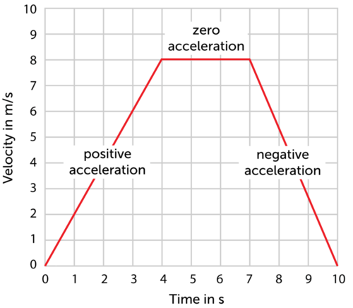
Introducing acceleration! Just like how velocity describes a change in position over time, acceleration describes a change in velocity over time. The equation to find acceleration is $a = \frac{\Delta v}{\Delta t}$. It should look familiar, since it mimics the form of velocity’s equation!

While there are semantic similarities between velocity and acceleration, they are not equivalent, and changing one has different effects on the overall motion of the object. For example, a velocity of 0 at a point in time means that the object is stationary. An acceleration of 0, however, supports no such conclusions, for all it means is that the velocity is constant. Now, the object could be stationary if the velocity was stuck at 0, but an acceleration of 0 does not convey that information. All you know, the velocity could be 0, 1, or -40.

Hmmm… can you do this same graph-shenanigans again? Absolutely! A change in acceleration over time is called jerk. A change in jerk? Snap! Then crackle and pop (seriously).

Position $\rightarrow$ Velocity $\rightarrow$ Acceleration $\rightarrow$ Jerk $\rightarrow$ Snap $\rightarrow$ Crackle $\rightarrow$ Pop

Unsurprisingly, you can look at the units of a measurement to determine what it actually is measuring (in the context of basic kinematics). Note, however, that the equations defining these properties support the units as well. Position can be considered to be the ‘base,’ so its unit of measurement is $m$. Velocity is a change in position over time, so $\frac{m}{s}$. Acceleration is a change in velocity over time, so it is $\frac{(\frac{m}{s})}{s}$, or $\frac{m}{s^2}$. Since we’re defining these properties to be the change of something over time, the ‘over time’ part cascades and results in higher and higher powers of $t$ the further up the derivative chain you go.